13-May-2015: Moment of Inertia of a Uniform Triangle

The purpose of this lab was to find the moment of inertia of a triangle about its center of mass using physical methods.

Part 1: Deriving our Theoretical Value:
To begin the lab, we first wanted to find an expression for the moment of inertia of a uniform triangle by derivation. To do this, we took two approaches.

In the first approach, we considered the triangle to rotate about the edge of its base. We found an expression for this moment of inertia and then used the parallel axis theorem(I_cm=I_{around one edge} + M(d_{parallel axis displacement})²) to find its moment of inertia about its center of mass. (see Fig. 1).

Fig. 1
Although the formula uses "b" as its term for the side perpendicular to the axis of rotation, this is actually the "height" of the triangle.

In the second approach, we considered the triangle to rotate about the edge of its height. We used the same method as we did in the first approach. (see Fig. 2)

Fig. 2
Using the same method as before, we altered the axis at which the triangle rotated.

Once we had derived from both approaches, we found that our expression for the moment of inertia about the center of mass of the triangle was going to be I= (1/18)Mb^2, where "b" is the base perpendicular to the axis of rotation.

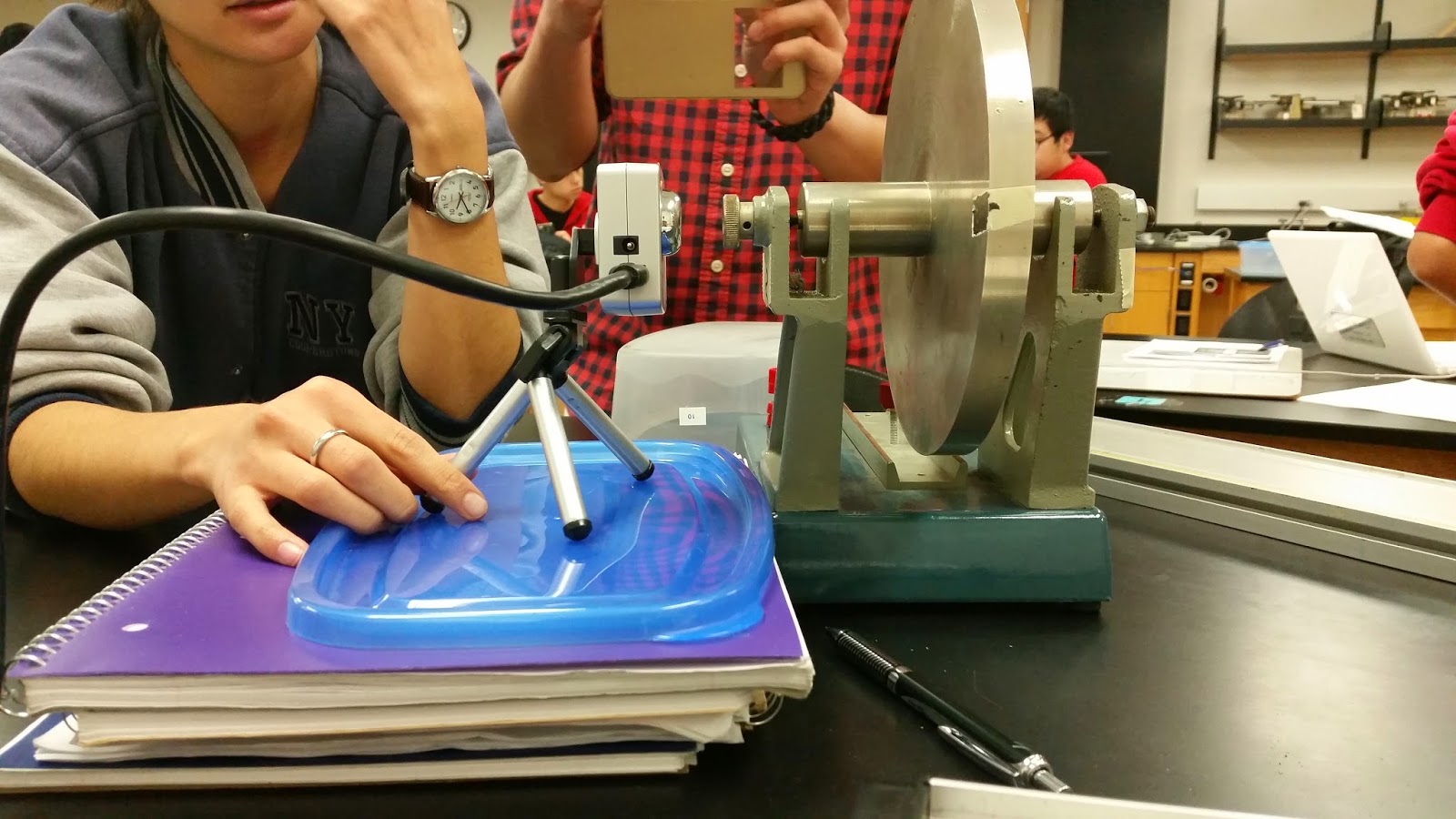
^{Part 2: Physically Finding the Moment of Inertia:Once we had our expression, it was now time to actually find the moment of inertia using the apparatus from our previous angular acceleration lab}. Using the formula I=(mgr/a)-mr^2. (a=angular acceleration), we could find the moment of inertia of the apparatus in three separate trials. We used a hanging mass of 25.0 g, and a torque pulley of 2.51 cm radius. The only information we needed was the mass that was being dropped and the radius of the torque pulley, given that LoggerPro would give us the angular acceleration of the system. 

The idea is that if we find the moment of inertia of the system by itself, and then the moment inertia of the system and the triangle (orientated either way), we could find the moment of inertia of the triangle by taking the difference of the two. 

We ran three trials: One without the triangle (moment of inertia of just the system), one with the triangle long-ways up (moment of inertia of the system and vertical triangle- Fig. 3), and one with the triangle long-ways down (moment of inertia of the system and horizontal triangle- Fig. 4). In each setup, we wrapped a string around the torque pulley and allowed the system to free fall. Using LoggerPro, we were able to find the angular acceleration of the system by taking the slope of the angular velocity vs time graph. However, since there is some friction in the system, we had to take the average value of angular acceleration (going up and down) as our usable value  (Fig. 5)

Fig. 3
We placed the triangle vertically up, giving us a specific value for the moment of inertia.

Fig. 4
The moment of inertia of the triangle would be the difference of its combined inertia with the system and the inertia of the system by itself.

Fig. 5-1
We needed to find the average angular acceleration in order to attempt to cancel out the torque due to friction.

Fig. 5-2

Once we had all of our angular accelerations, it was time to begin calculating the moments of inertia of each setup. (see Fig. 6) 

Fig. 6

We were left with a final moment of inertia of the center of mass of a triangle rotating about its vertical height being .00023902 kg*m^2. The moment of inertia of the center f mass of a triangle rotating about its horizontal base was .0005586 kg*m^2.

Once we had our theoretical values, it was time to find the percent error from the actual values. With our equations from before, we measured the height of the triangle to be 14.936 cm, its base to be 9.844 cm, and its mass to be 456 g. (see Fig. 7)

Fig. 7
The low % error showed that our expression for the moment of inertia was legitimate. 

We found that our percent error was less than 3% for both cases, which indicated that the experiment in all was a success and our expression for the moment of inertia of a uniform triangle was good in both cases.

Conclusion:
By deriving an expression for the moment of inertia of a uniform triangle around some axis and then using the parallel axis to find it about its center of mass, we were able to find a good prediction of a real physical attribute of this rotating triangle. Considering that the main source of uncertainty would be in the case of friction altering our angular acceleration, I believe that our % error being less than 3% is very reasonable.

11-May-2015: Moment of Inertia and Frictional Torque Lab

The purpose of this lab was to find the moment of inertia of a disk and use that determine the frictional torque that acted on it. We would then use this information to determine to solve an inclined cart problem.

Part 1: Finding the Frictional Torque:
The apparatus consisted of a large metal disk attached on a central shaft. The disk would spin on this shaft (see Fig. 1).

Fig. 1

To begin, we needed to understand what we were exactly looking for. Considering that the net torque is equal to the moment of inertia multiplied by the angular acceleration, we needed to find the moment of inertia of the entire rotating object first. To do this we needed to split the apparatus into three components: two shaft cylinders, and the main center disk. With the equation for the moment of inertia of a disk being I=(1/2)MR^2, we needed to find the radius of all three of the disks. To do this, we used calipers to precisely measure their diameters (see Fig. 2) and then divided this value by 2. Once we had the radii, we needed to find the mass of each individual piece. To do this, we used percent composition. That is, we found the volume of the disk and two cylinders, totaled it up, and found the percentage that each piece made of the whole. To find the volume, we simply found the thickness of each piece (see Fig. 3) and used the equation V=pi*r^2*h.If we had the percent composition, we could then find the percent composition of mass for each piece. On the disk was labeled the entire mass of all three components together. We broke this mass into the percentages we calculated and got our mass for each piece (see Fig. 4 for calculations).

Fig. 2
Measure the diameter of the disks, we used calipers to get a precise value, and then took a picture of the calipers reading to analyze it more thoroughly.

Fig. 3
Using the end of the calipers, we were able to measure the lengths of the smaller disks.

Fig. 4-1
Here we found the percent composition of the volume of the rotating apparatus. 

Fig. 4-2
We used the percent composition to determine the mass of each individual piece of the rotating apparatus.

Once we had our masses, we found the moment of inertia of the two cylinders and center disk, and then summed it all up. Our final moment of inertia of the entire apparatus was calculated to be 0.019986 kg * m^2 (see Fig. 5 for calculations).

Fig. 5

Once we had our moment of inertia for the apparatus, we then proceeded to find the deceleration of the disk due to its frictional torque. To do this, we set up a camera at one end of  disk, directly lined up with the central shaft (see Fig. 6). Once we opened LoggerPro and ensured that we were getting live video feed, we gave the disk a gentle spin and let it slow down to a stop.

Fig. 6
We lined up the camera to get an accurate visual of the disk.

Once we had our video capture, we went back to LoggerPro to analyzed the data. To do this, we placed a coordinate system into the video, placing our origin directly over the central shaft. From there, we marked one specific point on the disk and followed it frame by frame as the disk slowed down (see Fig. 7) NOTE: We placed a black piece of tape on the edge of the disk to clearly show the point which we were marking in LoggerPro.

Fig. 7
By placing dots at the black edge, we were able to obtain x- and y-coordinates for the position of the edge.

Once we had our points marked, we found that we had x- and y-components of velocity throughout the circular motion. Thus, in order to find our tangential velocity, we had to take the square root of the velocity in the x-direction squared and the velocity in the y-direction squared. We defined a column in LoggerPro to do this for us at every point (see Fig. 8).

Fig. 8
Using LoggerPro, we were able to find the tangential velocity at every point.

When we plotted the tangential velocity versus time, we found that the velocity had a downward linear like trend. Thus, in order to find the tangential acceleration, we found a linear fit for the graph. (see Fig. 9). This value for acceleration could then be divided by the radius of large center disk and found our value for angular acceleration (see Fig. 10).

Fig. 9
By finding the slope of the tangential velocity graph, we are able to obtain the tangential acceleration.

Fig. 10

With all of our calculation completed, it was now time to plug into our net torque equation to find the frictional torque of the system. When we multiplied our moment of inertia and angular acceleration, we found the net frictional torque to be -0.01808 (kg*m^3)/s^2. 

Part 2: Testing Our Value:

To test our value for the frictional torque, we set up an inclined cart system. This cart system would consist of a cart that would be attached by string to one of the small cylinders on the rotating apparatus. The cart would be placed on an inclined track, where it would be release from the top and allowed to roll down. The goal was to make a prediction for the amount of time it would take the cart to go down the track and then test that value (see Fig. 11)

Fig. 11
The cart would slide down the track while we recorded the amount of time it takes to reach the bottom.

First, we had to find an expression for the amount of time it would take the cart to go down the track. To do this, we combined our net torque and net force equations. We found the mass of the cart using a scale and the angle of inclination using our phones. (see Fig. 12 for full calculations) Our prediction was 7.95 sec.

Fig. 12

When we ran the actual experiment, we obtained a consistent value of 8.64 sec. This yielded us a percent error of 7.99%. The fact that the actual value of time was larger indicated that there were some forces that we did not account for, which is reasonable.

Overall, we were able to justify our value for frictional torque with our inclined cart test. However, some possible sources of error include our measurements, our ability to properly place precise dots on our video capture, and our ability to press our stopwatches in a timely fashion.

4-May-2015: Angular Acceleration Lab

The purpose of this lab was to find the relationship between the angular acceleration of a system, the force causing it to rotate, and the mass which is rotating. Along with this, we were to find the moment of inertia of our spinning disks.

Part 1: Relationships
To perform this lab, we set up rotating system that would comprise of two disks, a pulley, and a hanging mass. The idea was to attach the mass to the system by a string, have it attached some radius from the center of the disks, and allow it to fall. This would in turn cause the system to accelerate. We would then measure this in LoggerPro and record several trials with different hanging masses, disk masses, and rotating radii. (see Fig. 1).

Fig. 1
The apparatus consisted of a hanging mass, rotating disks, an air hose connected to an air valve and a rotational motion sensor.

To begin, we first had to measure all of the equipment we were planning on using. The materials included:

• Two steel disks (one for the top and another for the bottom)
• An aluminum disk (used to change the mass of the rotating disk)
• A small and large torque pulley (used to find the effect of changing the radius at which the force acts on the object)
• A hanging mass (used to cause the system to begin rotating)

Using calipers, we measured the diameter of the two steel disks, aluminum disk, and torque pulleys. (see Fig. 2). We then found the mass of the two steel disks, aluminum disk, torque pulley and hanging mass. (see Fig. 3) We recorded all this data on our white board.

Fig. 2
Using calipers, we were able to gain precise measurements of each disk. 

Fig. 3
Data Table

As seen in Fig. 1, the apparatus is hooked up to our laptop, allowing us access to data that LoggerPro could extract for us. The idea is that the black and white dashes around the disk could be counted while moving by some external sensor on the rotational apparatus. This would allow us to find angular velocity and acceleration. To properly set up the sensor, we had to input how many marks there were on the top disk (200). Once we had this, we were ready to begin collecting data. 

We tied the first mass (24.7 g) by string to the small torque pulley (r = 1.26 cm) atop the steel disk (1348 g). We began collecting data with LoggerrPro as we released the mass and allowed it to accelerate down. We collected data as the mass dropped and as it rose again, giving us an angular acceleration down (cw) and up (ccw). (see Fig. 4) However, we had to note that there was some friction within the system. The apparatus allowed for a virtually "frictionless" surface for the disk(s) to rotate, however in reality this was not true. Thus, in order to counter the effects of friction, we would simply take the average angular acceleration. This average acceleration is what we would use when analyzing and evaluating our data.

Fig. 4
The spike at the top of this graph indicates the turn around point of the hanging mass. To find the angular acceleration, we had to take the slope of this graph.

We ran the same experiment six times, with some slight changes each time. To find the effect of different tension pulling on the system, we ran the first three trials with the same small torque pulley, same top steel disk, but instead added additional mass to the hanging mass each time. To find the effect on using a different rotating disk on the system, we ran the next two trials with a large torque pulley, but with the top steel disk in one trial and the top aluminum disk in another. Finally, for the final trial, we used the large torque pulley and allowed the top and bottom steel disks to rotate. We received data through LoggerPro (see Fig. 5) and recorded it (see Fig. 6).

Fig. 5
Here are the graphs for all six of our trials. We took the slope of one only as an example.

Fig. 6

NOTE: During the data collection, we made an error when calibrating the machine to 200 marks per rotation. Our graphs represent angular accelerations that are slightly off. However, to correct the issue, we multiplied our values for angular acceleration by 360/200.

With all this data, we drew a couple of conclusions. First, we found that when we almost doubled the hanging mass, we almost doubled the angular acceleration. Same went for tripling the mass. Second, we found that when we used the large torque pulley rather than the small torque pulley (doubling the radius at which the tension acted on the disk) we also doubled the angular acceleration. Third, we found that when we decreased the mass of the rotating disk three-fold (using the aluminum disk rather than the steel disk) we INCREASED the angular acceleration roughly three times. Fourth, we found that when we doubled the rotating mass (allowed two steel disks to rotate), we cut the angular acceleration in half.

The final step in part one of this lab was to find the relationship between the linear velocity of the hanging mass and the rotational velocity of the system. To do this, we simply ran one run the exact same way as we did the other six trials. We used a large torque pulley for the tension to act on. The mass of the disks spinning and mass falling become irrelevant, as we are simply analyzing velocity in the angular and linear sense. Using a motion sensor and note card, we began collecting data with logger pro, in both rad/s and m/s. When we graphed linear velocity in the y-axis and rotational velocity in the x-axis, we obtain the graph in Fig. 7. When we took the slope of this graph (positive or negative), we obtained a value of 0.02513 m which translates into 2.513 cm, which is practically exactly the radius of the large torque pulley.

Fig. 7
We found that the slope of the linear vs angular velocity was exactly the radius of the large torque pulley.

Conclusions for Part One:

For part one of this lab, we were able to verify the magnitude of the hanging mass and the radius at which a force was acting on a disk were directly related to the angular acceleration of the system. This meant that if we increased the hanging mass, we increased the angular acceleration. (same for radius). We were also able to verify that if we increased the mass that was rotating, we decreased the angular acceleration. All of these relationships were numerically proportional (ie. if you double the hanging mass, you double the angular acceleration and if you tripled the mass that was rotating, you cut the angular acceleration into 1/3 of what it used to be). As for linear and angular velocity, we found that they were related by the radius at which the force acting on them was being applied. Through this, we were able to verify the relationship v=rω.

Part 2: Moment of Inertia of Each Disk:

For the second part of the lab, we had to use our tools to find the moment of inertia of the single top steel rotating disk, the two steel rotating disks combined, and the top aluminum disk. To do this we had to derive an expression for the moment of inertia of this system using the force and torque equations. We are finally left with the equation I=(mgr/α)-mr^2 To verify if this is true, we used the given equation for the moment of inertia of rotating disk as our "actual" value. I=(1/2)MR^2 Our calculations can be seen in Fig. 9

Fig. 9

In all, we found that we had a percent error of less than 5% for the single steel disk, both steel disks, and aluminum disk. This indicated that our data and formula were good. 


Conclusion:In all, the lab was a success and allowed us to find the multiple relationships between angular acceleration and the factors that change it. We were also able to verify our equation for the moment of inertia of a rotating solid disk with our data. However, we had to account for a few areas of uncertainty. This included all our areas of measurements as well as the frictional torque we did not account for. We assumed that averaging the angular acceleration would completely rid the friction, which is not entirely true. However, in all we were able to prove our moment of inertia and relationships.

22-April-2015: Collisions in Two Dimensions

The purpose of this lab was to determine whether not momentum and energy are conserved in a two-dimensional collision.

Set Up:

Intro:

To perform this lab, we needed two create an environment in which we could create, observe, and analyze a two dimensional collision. The collision would occur between two marble in two separate trials. The first would consist of two marbles with similar masses and the second would consist of two marble with different masses. To create a reasonable surface to conduct the lab, we used a leveled glass table. The idea was that we would leave one marble stationary at the center of the leveled glass table and another marble would be aimed directly at the stationary marble. Once ready to begin collecting data, we would flick/push our marble towards the stationary marble. Ideally, the balls would deflect off each other at some angle from one another. Theoretically, we should be able to conclude whether not momentum in the x- and y-directions was conserved and whether or not energy was conserved.

Actual Apparatus:

We setup the experiment just as describe above, with a leveled glass table and two marbles of similar mass and two of different. To observe and collect data from the collision, we had a camera setup directly above the leveled glass table. This camera would be hooked up to LoggerPro and would allow us to split up the velocity of the marbles into x- and y-components. This would in turn allow us to find the momentum in the x- and y-directions (Fig. 1)

Fig. 1
With one marble stationary, we would flick another marble at it and record the collision with our LoggerPro camera.

Part 1- Two Marbles of Similar Mass:

Fig. 2
When setting our origin, we tried to line up at least one axis with the path
of the flicked marble. This would leave us with only one value of velocity to
calculate in our initial stages before the collision. 

To begin the lab, we first  used the apparatus with two marbles of similar masses. The first marble, which we will call marble one, was measured to be 0.021 kg. The second marble, which we called marble 2, was measured to be 0.019 kg. We could conclude that these two marbles had relatively similar masses. As stated in the intro, we needed to flick one marble at the other while recording the collision. Once we were ready, we began collecting data and performed the collision. We analyzed the video capture in LoggerPro (see Fig. 2).

Fig. 3
This position graph shows us the position of the two marbles
 in both the x- and y-directions.

To analyze the video, we needed to set a scale and origin for the collision. Our scale was placed in the top right corner of the glass table, where we measured a small piece of it to be roughly 22.3 cm. We placed the origin at the stationary marble and attempted to line up the y-vertical axis to the path the flicked marble took. We then placed frame by frame dots at the positions of the marbles before and after they collided. We flicked marble one at marble two.

Once we analyzed the video, we were given enough data two obtain the graphs of velocity and position in both the x- and y-positions for the two marbles (see Fig. 3). For our trial, we would be mainly using the position versus time graphs. To find the momentum and energy of the marble, we needed to find the velocities before and after the collision in both the x- and y-directions. To do this we simply took the slope of the position graphs (see Fig. 4).

Fig. 4
If we found the slope of the position graphs, we could find our velocity in the x- and y-directions for both of the marbles.

Once we had the velocity of the two marbles, it was now time to manually calculate the change in momentum and kinetic energy of the two marbles. For momentum, we broke the problem into x- and y- components (see Fig. 5). For kinetic energy, we simply found the resultant velocity of the x- and y- velocities and used this value in the equation KE=(1/2)*m*v^2. (see Fig. 6).

Fig. 5
Calculations for the initial and final momentum. We lost 28.6 % of our initial momentum after the collision.

Fig. 6
 Calculations for the initial and final energies. We lost 64.7 % of our kinetic energy after the collision. 

Once we had our initial and final values, we compared our values for initial and final momentum and energy. In both instances, we wounded up with less in the final stage, which is reasonable given the fact that there are more forces acting on this system than we are accounting for. This will be further discussed in the error section.

Part 2- Two Marble of Different Masses:
The second part of the lab included the same apparatus, only this time the two marbles would have different masses. We would flick a small marble (0.005 kg) at our original marble one (0.021 kg). Once again, we captured the collision on video and analyzed it on Logger Pro.

Just like before, we set our origin, scale and points on the video. This in turn would allow us to analyze the velocity of the two marbles. Just like before, we were planning to use the slope of the position graphs to find our initial and final momentum and energy (see Fig. 7)

Fig. 7
Again, we found the slope of the position graphs to find our values for velocity.

Once we had our values for velocity in the x- and y-directions for both of the marbles, we then found the initial and final momentum and kinetic energy for the system (see Fig. 8)

Fig. 8
Once we had our values for velocity, we calculated our momentum and kinetic energy for the collision.

Again, we found that we had lost some energy and momentum in our collision, however, this may have been due to the error in our lab.

Conclusion and Error:

As we can see from the collected data, energy and momentum was not perfectly conserved in this collision. This may have been due to the following sources of error in our lab:

• The surface of the glass table and marble were not completely frictionless, which suggests the presence of an external force.
• As we can see Fig. 2, the video capture did not give us an accurate image of the collision. Instead, it was slightly curved. This may have altered our ability to find the true position of the marbles. 
• Again with the video capture, the marble moves quickly enough to make it difficult to find its pin point center in every frame, causing there to be some uncertainty in its position.
• All of these values become estimates as the sources of error pile on.

However, although we had all these sources of error, are results are relatively realistic. In every instance, the difference in energy and momentum is a loss, which in a real life situation is probable. Overall, in a perfect world this lab would have yielded us a more accurate depiction of the conservation of momentum and energy.

27-April -2015: Ballistic Pendulum Lab

The purpose of this lab was to find the initial velocity of some mass in a ballistic pendulum by combining both conservation of momentum and energy.

Setup:

Fig. 1
The setup

Unlike most of our other experiments, this lab was initially setup and ready to go the day of our lab. The apparatus consisted of a ballistic pendulum to which a spring gun was aimed at. From the spring gun a small mass projectile would be shot out. When done correctly, the mass would become lodged in the pendulum, causing it to swing upwards and to the right. The angle displacement of the pendulum could then be read by a protractor attached to the apparatus. Beginning at zero degrees from which the pendulum was stationary, the protractor would swing upwards as the pendulum pushed, and would then stay in place as the pendulum swung back. This would give us the angle of displacement. (see Fig. 1 and Fig. 2 for setup)








Measuring Data:
Once the projectile was loaded into the spring gun, we cocked the spring back, allowed the ballistic pendulum to be completely still, and FIRED! As expected, the pendulum swung to the right and was displaced by some angle. All we could measure from this was the angle of displacement, which measured to be 17.2 degrees (+/- 0.1 degree) and the length of the string(L) which was 21.7 cm (+/- 0.1 cm)

Fig. 2
The ball was lined up so that it would fit snug into the pendulum.

Calculating Initial Velocity:
We only had two equations at our disposal that we could have used to calculate the initial momentum of the projectile: Conservation of Momentum and Conservation of Energy equations. (NOTE: We were given the mass of the projectile(7.63g +/- 0.01g) and the mass of the ballistic pendulum(80.9g +/- 0.1g) For the conservation of momentum, we were missing the initial velocity of the projectile and the final velocity of the projectile and pendulum (see Fig. 3)

Fig. 3
We had to come up with an expression for the final velocity of the system.

Since our end goal is to find the initial velocity of the ball, we had to come up with an expression for the final velocity of the ball and pendulum. This is where our conservation of energy equation comes into play. Conceptually, we know that the initial energy will only consist of the kinetic energy of the ball and pendulum, and the final energy (gravitational potential energy) we would consider at the maximum height of the pendulum. (see Fig. 4 and Fig. 5)

Fig. 4
To calculate the height at which the pendulum went, we had to do some trigonometric work.

Fig. 5
Our final expression for the velocity of the system after initial impact.

Once we had our expression for the velocity of the ball and pendulum, we could plug that back into our original momentum equation. (see Fig. 6) At this point we could simply plug in our values for the mass of the ball, mass of the pendulum, length of the string, and the angle at which it was swung. This would eventually give us an initial velocity of 5.06 m/s. (see Fig. 7)

Fig. 6
Our final expression for the initial velocity of the ball.

Fig. 7
We found our initial velocity to be 5.06 m/s BEFORE finding our uncertainty.

Calculating the Propagated Uncertainty:

Although we had our value for the initial velocity of the projectile, we had to account for the fact that all of our measurements had some uncertainty. To do this, we did propagated uncertainty (see Fig. 8 for all calculations).

Fig. 8
Calculating the uncertainty in our entire expression.

Our final answer came out to be 5.060 m/s +/- 0.052 m/s for the initial velocity of the ball. The only major sources of uncertainty occurred when we had to read the measurement of something with our naked eye (ruler for length and protractor for angle). Other than that, however, our answer came out to be fairly accurate.

15-April-2015: Impulse-Momentum Activity

The purpose of this lab was to prove the Impulse-Momentum Theorem: The change in momentum is equal to impulse.

Part 1: Elastic Collision:
Setup:

Fig. 1

To set up this lab, we needed a few materials:

• Two carts, one with an extended spring.
• A track that would direct one of the carts.
• LoggerPro, force sensor, motion sensor.
• Rod and some clamps.

First, we secured the cart with the extended spring to the lab bench using the rod and some clamps. Once we had done this, we setup up the track into such a way that a cart moving on the track would collide with the stationary cart attached to the lab bench. Once we had this, we attached the motion sensor to the cart which would move on the track, facing the direction of impact. Finally, we hooked up a motion sensor at the opposite end of the track (see Fig. 1 for set up).

Conducting the Experiment:

Once we had our setup complete, it was time to begin the experiment. First, we zeroed our force sensor in both the horizontal and vertical direction. Once this was done, and LoggerPro was ready with both sensors, we began collecting data and gave the cart a gentle push towards the stationary cart. The cart collided and repelled back.

Analyzing Data:

To test the impulse-momentum theorem, we first had to calculate the change in momentum. To do this we first found used logger pro to find the initial velocity of the cart and the final velocity of the cart. By taking the mean value of the velocity of the cart before and after the collision, we would be able to find both initial and final momentum of the cart (see Fig. 2). The mass of the cart we measured to be .678 kg. Thus the change in momentum = mv(f)-mv(o). = .678(-0.3965-0.4796)= -0.594 kg*m/s.

Fig. 2
After we had completed the lab, we found that one of our runs had been misplaced. During lab, we obtained the real values for initial and final velocity, however the graph from which we obtained it from had been deleted or altered. Thus, Fig. 2 contains a sample graph of what it the velocity graph for the first trial should have looked like. THIS IS NOT THE ACTUAL GRAPH.

For Impulse, we took the area under the Force vs Time graph (since we knew that Impulse= F*t, or the integral of F*dt.) and found that to be -0.6137 N*s. (see Fig. 3) With a 3.2 % difference, we could confirm the impulse-momentum theorem (see Fig. 4 for all calculations).

Fig. 3
Since we did not reverse the direction of the force sensor, we obtained a negative force, which in turn gave us a negative impulse.

Fig. 4
We compared our calculated impulse to that of LoggerPro's and found that the two values were reasonably close.

Part 2: Elastic Collision with More Mass:

Fig. 5

It was now time to conduct the experiment with the same setup, only now we added more mass to the moving cart. The goal of this trial was to determine whether or not the mass would affect the overall outcome of the impulse-momentum theorem.

With the exact same set up, we simply added 0.2 kg to the cart (see Fig. 5). Once again, we gave the cart a slight push, and collected data using LoggerPro. 

We found the initial and final velocity of the cart, which in turn lead us to the initial and final momentum of the cart. We took mean of the velocity graph before and after the collision which gave us an estimate of both the initial and final velocities. Our new cart mass was .878 kg. However, in this trial we added a magnetic mini white board to the back of our cart (this was to allow the motion sensor to track the cart more easily). The mass of the mini white board was .072 kg, which lead to a new total mass of 0.950 kg. We calculated our change in momentum to be -0.883 kg*m/s.

We again used LoggerPro to integrate the area under the Force vs Time graph and found the impulse to be -0.8537 N*s. There was 3.2% difference between the values. (see Fig. 6 for graphs, and Fig. 7 for calculations). This again confirmed the Impulse-Momentum Theorem.

Fig. 6
Since the velocity was relatively constant before and after the collision we were able to find the mean of the two horizontal pieces to find a reasonable value for momentum.

Fig. 7
Again, we were able to confirm the impulse-momentum theorem due to such a minimal difference between our change in momentum and impulse.

 Part 3: Inelastic Collision:
For the third portion of the lab, we wanted to examine the impulse-momentum theorem under inelastic conditions. To do this, we change our setup slightly. We replaced the stationary spring cart with a secured wooden block. Attached to this wooden block was a piece of clay. We then replaced then added a rubber stopper to the end of our force sensor, to which we attached a nail.The nail would then attach to the clay upon impact, not allowing the cart to bounce back. This would make our inelastic collision. We left the motion sensor and track as was (see Fig. 8).

Fig. 8

Once all of our equipment was set up, we once again gave the cart a slight push and began collecting data. With the cart being stuck to the clay upon collision, we knew the final velocity would be zero. Thus, we were only left to find the initial momentum. Since our graph gave us a slight downward slope, we tried to use the velocity most near the moment of impact, since this would be considered the initial velocity (see Fig. 9).

Fig. 9
Since the velocity is not reasonably constant, we measured the velocity 
nearest the point of collision.

Once we had this, we calculated our momentum. For this trial, we left the added mass on the cart and added the mass of the nail and rubber stopper which totaled to be 0.967 kg. We found our initial momentum to be 0.3733 kg*m/s, which meant our change in momentum was -0.3733 kg*m/s. We once again used LoggerPro to calculate the impulse exerted on the cart (see Fig. 10).

Fig. 10
We again used LoggerPro to calculate impulse using our Force vs Time graph.

We found this to be -0.305 N*s. (Note that we did not include the integral beyond the initial impact. The other humps in the graph were due to the vibration of the cart once it initially hit the nail. We compared the impulse we calculated to the impulse LoggerPro calculated and found that the values had a 20.1% difference (see Fig. 11 for all calculations).

Fig. 11
For our inelastic collision, we found that the difference between our change in momentum and impulse was significant. This indicates that there was some possible source of error. This could be explained perhaps due to the fact that velocity was not completely constant and there was some significant outside force(friction) acting on the cart.

Error, Comparison, and Conclusion:

When comparing the Force vs Time graph of the inelastic and elastic collisions, we found the they were similar in height, but different in thickness. Since we kept the extra mass on the cart for the inelastic collision, we compared the Force vs Time graph in Fig. 10 to that in Fig. 4. The thickness of the elastic collision force curve was much larger than that of the inelastic. 

There were quite a few areas of uncertainty in our lab. For one, we could not get any of the trials to a perfect constant initial velocity. This was especially apparent in our inelastic trial, in which the slope of the velocity graph is extremely apparent. However, perhaps the most prominent source of error was our inability to create a perfectly inelastic or elastic collision. This prohibited us from obtaining perfect results.

Once completed with the lab, we had verified the impulse-momentum theorem for both elastic and inelastic collisions. The elastic collisions had a small percentage difference between the different impulses, while our inelastic collisions had a rather large one. However, we believe that the larger gap may have been due to the fact that we did not give the cart a sufficient enough push and the added fact that the cart vibrated back and forth after colliding with the clay.